Connect X: MCTS vs. Minimax
Empirical study comparing Monte Carlo Tree Search and Minimax in Connect X.
Abstract
Connect X, a solved perfect-information strategy game, has established itself as a staple in game AI research. With the rise of advanced non-machine-learning search techniques like Monte Carlo Tree Search (MCTS), traditional methods such as heuristic Minimax are struggling to maintain their relevance. This study offers an empirical comparison of these approaches using both result-oriented and result-agnostic metrics to assess their performance in a Connect X setting.
Introduction
The arrival of Monte Carlo Tree Search (MCTS) has transformed the field of game AI, notably through its integration with AlphaGo
Background
Connect X
Connect X is a two-player game traditionally consisting of a board of 7 vertical slots containing 6 positions each. Both players alternate to choose a slot to drop a chip that falls to its lowest free position. The goal is to attempt to create horizontal, vertical, or diagonal chip sequences of given length $ X $.
Minimax Search
Minimax Search, introduced by Von Neumann in 1928
Monte Carlo Tree Search
Monte Carlo Tree Search (MCTS), introduced by Kocsis et al.
Methods
Minimax Implementation
The Minimax algorithm was implemented recursively, with each tree node invoking the same function on its successors. Although an explicit tree data structure was constructed during the algorithm’s execution, this was optional and primarily done for evaluation purposes. It is worth noting that implementation variations that do not construct this tree may yield different results for metrics like the time taken to pick a move. Additionally, alpha-beta pruning was integrated to reduce the search cost, improving the algorithm’s efficiency.
Evaluation Function
The evaluation function implemented to guide the Minimax search was heavily inspired by the literature, specifically by the work of Kang et al.
| ID | Sequence | Explanation | Utility |
|---|---|---|---|
| 1 | $X$ | Winning state. | inf |
| 2 | $X-1$ | 2.1 Spaces available at both sides. | inf |
| 2.2 Space available at one side. | 90000 | ||
| 2.3 Spaces available at neither side. | 0 | ||
| 3 | $X-2$ | 3.1 Spaces available at both sides. | 50000 |
| 3.2 Spaces available at one side. Depends on number of spaces available ($s$). | $\max(0, (s-1) \times 10000)$ | ||
| 3.3 Spaces available at neither side. | 0 | ||
| 4 | 1 | Depends on chip's distance to center column ($d$). | $\max(0, 200 - 40 \times d)$ |
The function can be broken down into 4 distinct features, as shown in the table above. Each feature corresponds to the presence of chip sequences of length $X$. Moreover, each feature is comprised of sub-cases that will help to determine the value of a given game state. The most important feature is 1, which returns a value of infinity on the winning terminal nodes, as no other state is more valuable. The function $E$ will be calculated for the perspectives of players that maximize ($max$) and minimize ($min$), with a final value of $E(max) - E(min)$ to balance out the resulting heuristic value.
For simplicity, the figure below will be used to explain the subcases of feature 2 in a game with board dimensions [6, 7] and $X=4$. Assuming that red is $max$, $E(max)$ would yield infinity for the leftmost state, since a win is unstoppable at that point (2.1). The middle left state would result in 90k, as it represents an immediate advantage/threat (2.2). On the other hand, both the middle-right and right-most boards would yield 0, as the former cannot lead to a win, and the latter does not have any immediately available moves on either side (2.3). This is done to ensure that the $E$ does not overestimate a state’s utility.
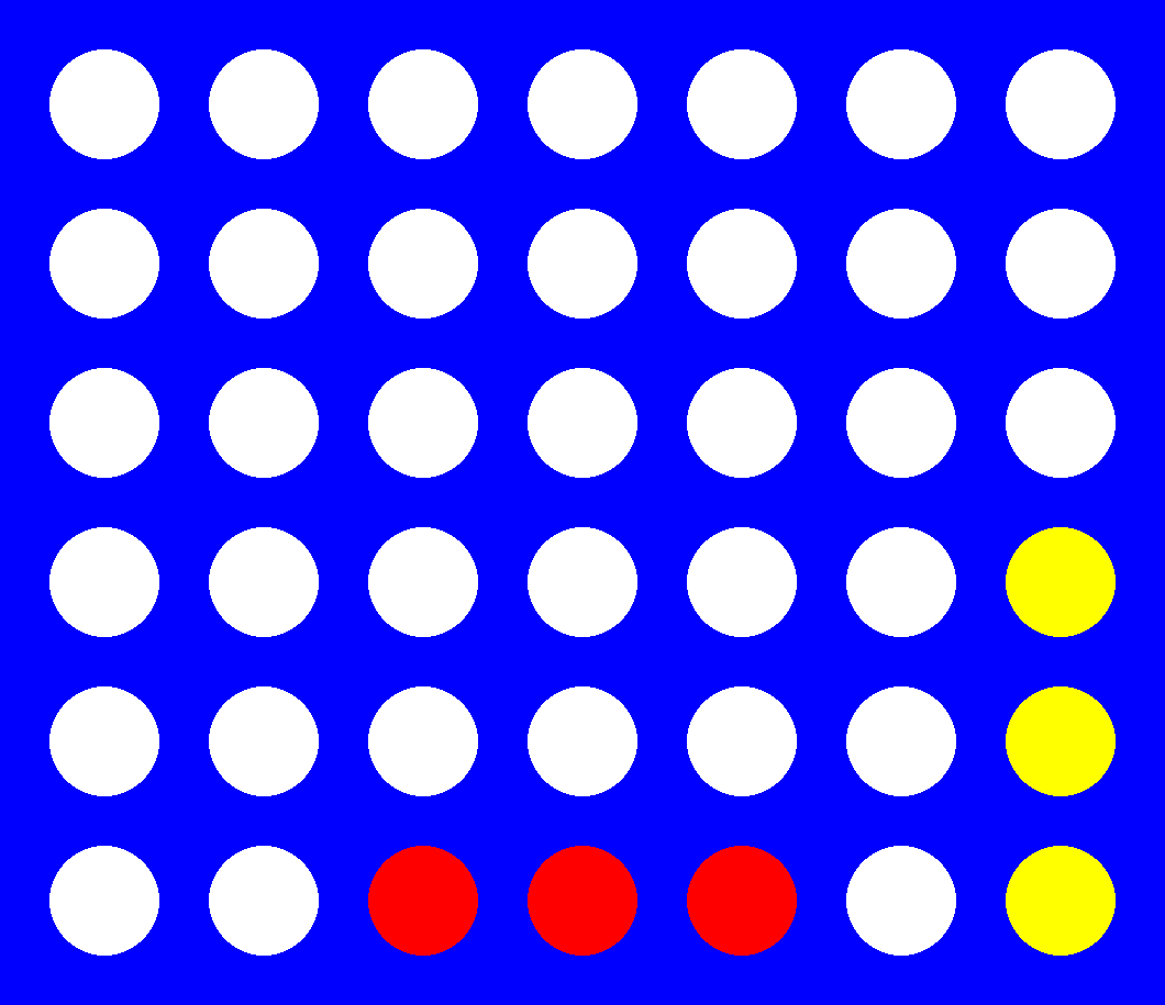
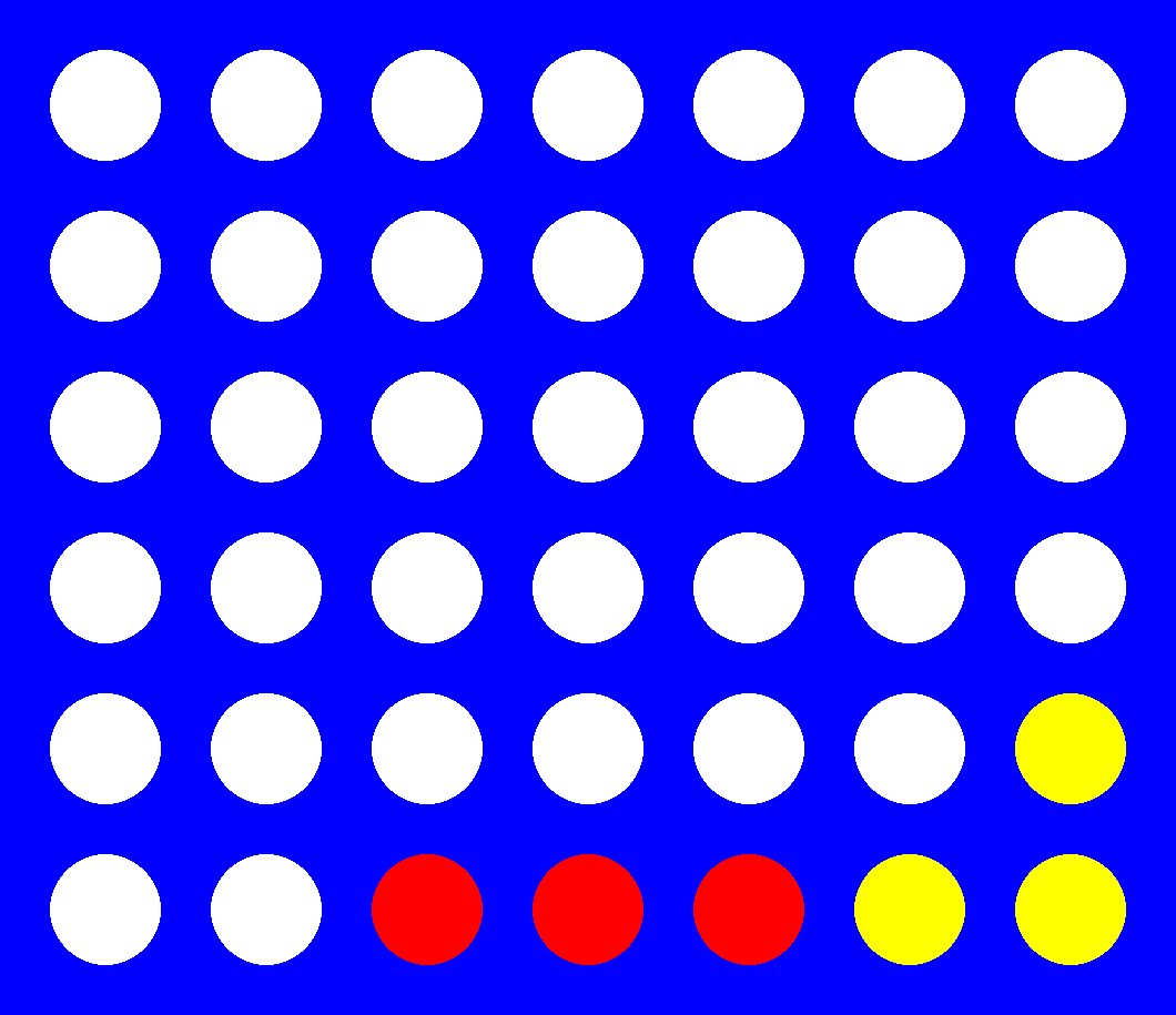
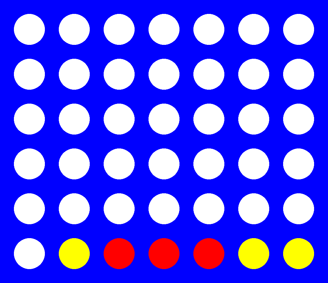
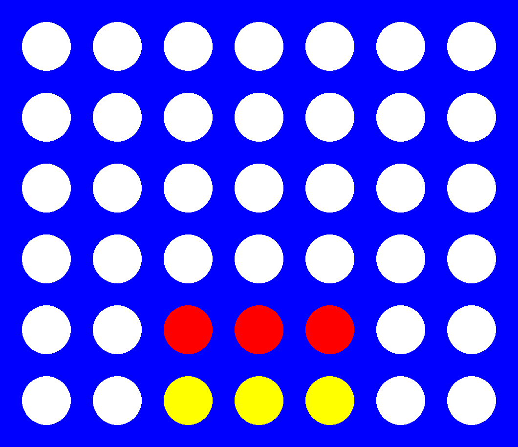
Feature 2 examples.
Note that E yields a value of 0 when there is a single available space (s = 1) on one of the sides of a C-2 sequence (3.2). The equation:
is proposed as it guarantees a utility of 40k for the case of 5 available spaces, the maximum of a traditional board of 7 columns, while still being lower than 3.1. Reasonably, one could argue that this might not scale well to different board sizes, which is recognized as a weakness of feature 3.2. In contrast, feature 4 will return a much lower value, as it is significantly less powerful than the other combinations. Chips closer to the center have a higher utility as they provide an increased number of potential plays being further from the edges of the board.
In terms of implementation, heavily optimized convolution operations were used to facilitate the detection of chip sequences of given lengths throughout the board. The convolution kernel employed consisted of all zeroes, except for the locations corresponding to the sequence being targeted, where ones were placed.
Empirical Comparison
Since Minimax search would theoretically be able to expand the entire game tree at each move to assess every possible state, four distinct computational budgets were set to ensure a fair comparison. The budget refers to Minimax’s game state evaluations (tree nodes) and MCTS’ game tree rollouts. Since Minimax’s budget consumption depends on its depth parameter, different depths are assessed. On the other hand, since the number of MCTS’ rollouts is budget-agnostic, three different strategies were proposed to control its consumption behavior:
- Thrifty: Allocates the same budget to every move, assuming a game with $rows \times cols$ chips dropped.
- Optimistic: Allocates a budget of 1 to the last move, with uniformly increasing budgets for earlier moves. This agent is optimistic about the possibility of winning earlier with a larger budget.
- Greedy: Allocates the entire budget equally among the first half of potential moves, leaving no budget for the second half.
When an agent runs out of computational budget in the middle of a game, it forfeits, and its opponent automatically wins. Note that Minimax will have depth number of additional moves after its budget is consumed, since it can reuse the tree computed in previous moves without further state evaluations.
Two main simulation sets were run to empirically compare both algorithms. Sets consist of 12k and 19k total simulations, respectively. Both involved running a number of repeats per unique combination of hyper-parameters to ensure fairness in the assessment of both agents. The hyper-parameters in question were: first set: depth, starting agent (to get rid of a possible source of bias), budget, and MCTS strategy; second set: board dimensions (and X values), budget, MCTS strategy, and starting agent. Additionally, depths were not included in the second set as only the best-performing ones were selected to compete (results from the first).
For every move, relevant metrics and game attributes were recorded in a parquet file that was later used for the analysis. Some of these metrics included: time (ms), number of tree nodes, current agent, etc.
Results
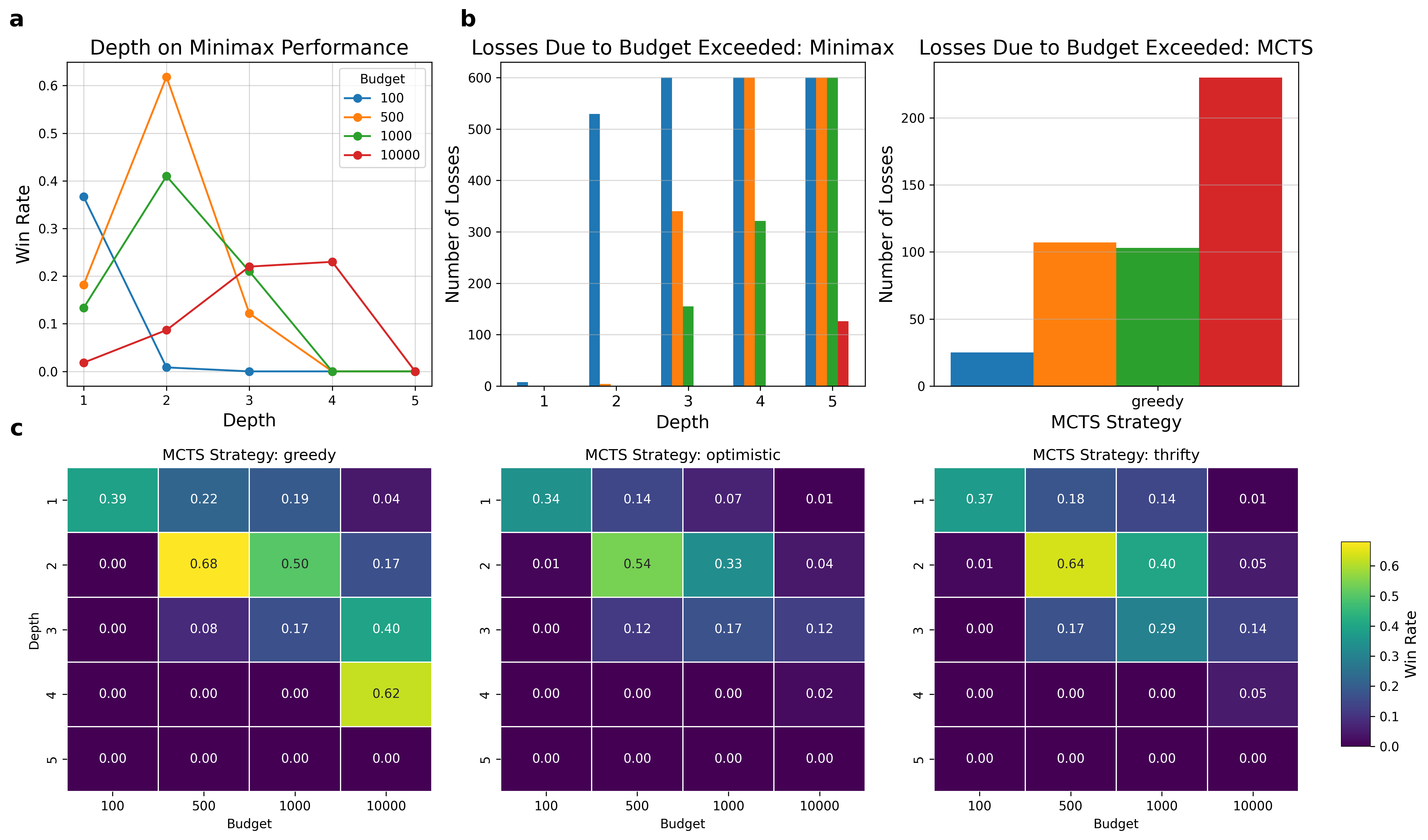
a, b, c, Analysis of game results. a, Line plot of the effect of Minimax's depth on its (adjusted) win rate across multiple budgets. b, Bar plots of number of losses due to forfeit/budget depletion across multiple budgets. Color scheme follows that of a. Left: Comparison of Minimax depths. Right: Greedy MCTS. c, Heatmaps of Minimax's win rate across multiple depths, budgets and MCTS strategies. Each map represents a strategy. Color scheme maps win rate.
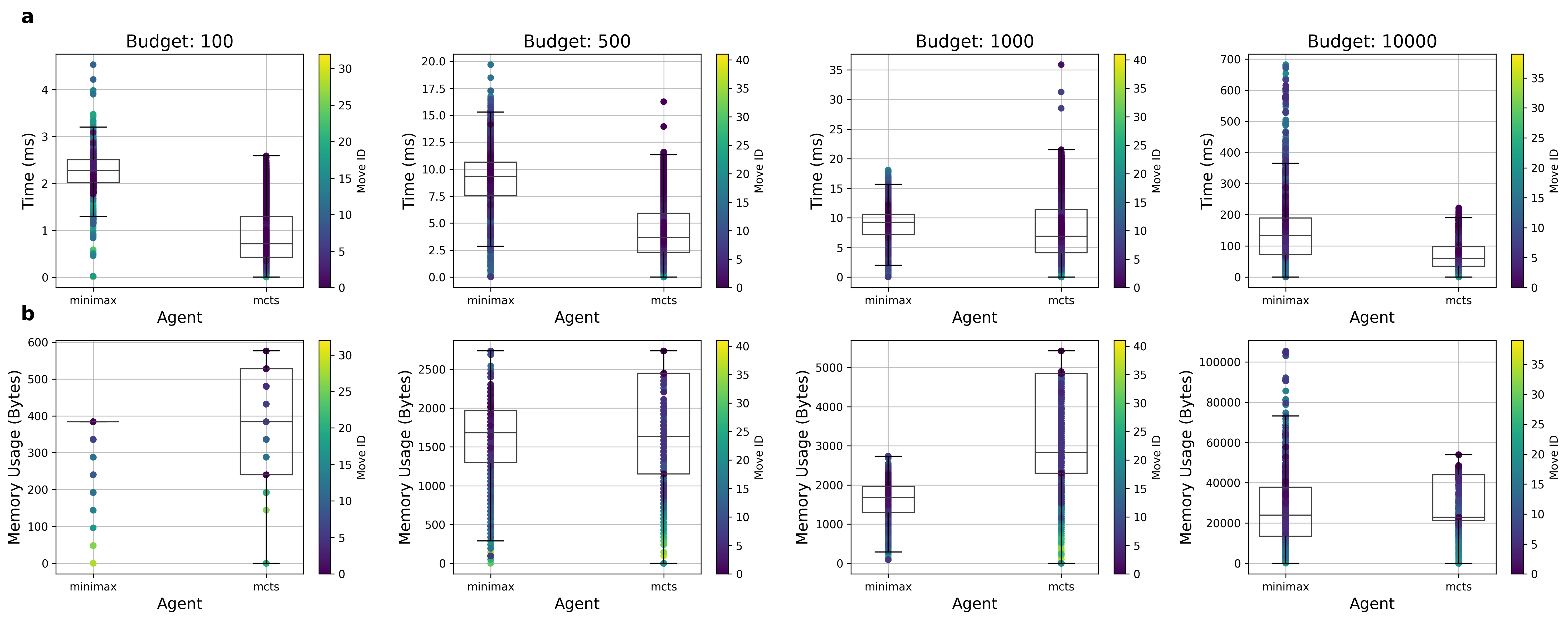
a, b, Visualization of result-agnostic performance metrics. Only Minimax's best depth at each budget. Color scheme represents the timing of each move, indicating how early or late in the game it was performed. a, Box plot visualization of time (ms) taken to pick a move across all budgets. b, Box plot visualization of approximation of memory (bytes) consumed at each move. Calculated as $mean(Minimax Node (bytes) \div MCTS Node (bytes))$.
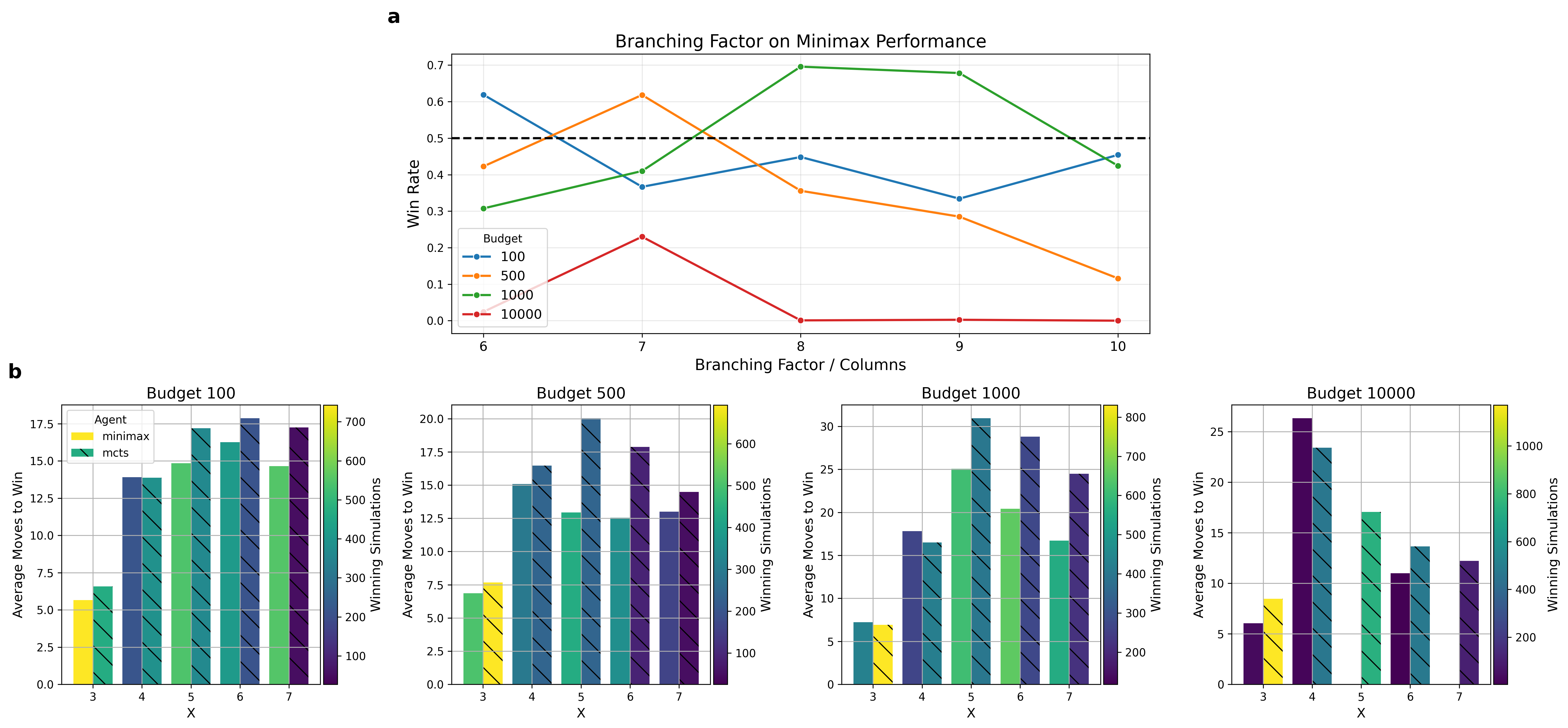
a, b, Simulations extended to variable board/rule configurations. Again, Minimax's depths at each budget were chosen according to the previous analysis. a, Line plot visualization of the effect of the game's branching factor (board's number of columns) on Minimax's win rate across multiple budgets. The dashed line marks the 50% win rate, with every point above it indicating performance superior to that of MCTS. b, Bar plots showcasing the average number of moves played to reach a win across X values. Every plot represents a budget, the color scale indicates the number of simulations used to compute the average, and the hatch indicates the agent.
Discussion
As evidenced from the results, the number of losses due to budget depletion is inversely proportional to the win rate for any given budget, which aligns with theoretical expectations. The optimistic MCTS performed the most consistently across multiple budgets and depths, followed by the thrifty and greedy. The heatmaps reveal that the choice of MCTS strategy is crucial. Although the idea of a greedy agent was appealing, particularly for larger budgets, games tend to take longer when agents can afford to utilize more computation, which resulted in a significant number of greedy losses due to budget depletion. On the other hand, it is pleasing to see that the optimistic agent performed relatively close to expectations. Since the game tree is significantly bigger at early stages–as will be explained later–the higher initial budget allows for MCTS to build a better foundation of chips.
Picking moves at later stages of the game requires less memory for both algorithms, which aligns with a decreasing branching factor for the states in question. However, no clear patterns emerged concerning the time taken to pick a move and its timing–how late or early in the game the move was played. Moreover, MCTS built overall larger game trees in most budgets, which could explain its higher win rates. In fact, the only case where Minimax’s mean memory consumed was significantly higher (budget 500) is also the case where Minimax could win more games than its Monte Carlo counterpart. One could think of this budget and depth combination as a ``sweet spot’’ in Minimax’s favor, where the richest trees were able to be generated without risking computation depletion. Moreover, the growth in time and memory is exponential with respect to depth and budget for both agents.
For the second set of simulations, one could state that MCTS generalized better across different board and rule configurations. However, it was surprising to see Minimax achieve really high win rates for some of these new combinations. Focusing on the three cases mentioned before, one could transfer the information gathered from the result-agnostic box plots to affirm that increasing the branching factor allowed for a Minimax algorithm that fully utilized its computational budget (since a higher branching factor would result in bigger game trees), specializing in outclassing MCTS for said combinations (around 70% win rate). Moreover, one could state that Minimax performs better at really low budgets and small boards, since terminal states are reached faster. On the contrary, MCTS shines at higher computational budgets, particularly when paired with larger board sizes. Interestingly, the weakness identified on feature 3.2 did not really hold in practice, as budgets 100 and 1k didn’t appear to perform significantly worse for bigger board sizes.
It is safe to say that Minimax is more efficient with its wins, as it is shown that fewer numbers of moves are needed to end a game. This could be interpreted as $E$ being either really accurate of a game state’s utility or, alternatively, relatively poor.
Conclusions
MCTS proved to be generally more effective in terms of time and memory consumption. Note that, in this case, higher memory usage is desirable as it indicates that the computational budget is being utilized to its full potential. As demonstrated by the data collected, MCTS was also the superior search algorithm in terms of game results, with some interesting exceptions.
A limitation of this study lies in the decision to include all MCTS strategies in the analysis. It is reasonable to think that this approach may not have been entirely fair to MCTS, as the optimal Minimax depths were tailored for each budget. This choice was motivated by a conflict between the optimal Minimax depth and the best-performing MCTS strategy, as these configurations rarely align. Moreover, while Minimax depths were strategically selected to minimize defeats caused by budget depletion, this risk remained present, particularly with bigger board sizes. On the other hand, selecting a specific MCTS strategy that avoids such losses (e.g., thrifty or optimistic strategies) could be perceived as unfair to Minimax.
Future extensions of this study could involve exploring alternative MCTS strategies or refining the evaluation function. Otherwise, another direction might be redefining the budget’s nature to reflect more realistic measures, such as time allowed to pick a move or CPU utilization.
Enjoy Reading This Article?
Here are some more articles you might like to read next: