Classifying CIFAR-10

We tackled the task of classifying CIFAR-10 images by comparing multiple supervised learning approaches. You can access the Jupyter notebook in the repo.

Supervised machine learning is a widely used form of artificial intelligence. There are many approaches to supervised learning, including Neural Networks, Convolutional Neural Networks, and Residual Networks.

CIFAR-10

CIFAR-10, a subset of CIFAR-100, consists of 60000 32x32 colour images split into 10 classes (6000 images per class). There are 50000 training images and 10000 test images.

Linear Neural Network

To begin with, let’s start with a simple deep NN of 5 layers with no activation function on the last layer. We will be using ReLu to introduce non-linearity.

As simple as:

class MyNN(nn.Module):
  def __init__(self, ni, nh1, nh2, nh3, nh4, no):
    super().__init__()
    self.layer1 = nn.Linear(ni,nh1)
    self.layer2 = nn.Linear(nh1, nh2)
    self.layer3 = nn.Linear(nh2, nh3)
    self.layer4 = nn.Linear(nh3, nh4)
    self.layer5 = nn.Linear(nh4, no)

  def forward(self, x):
    x = torch.relu(self.layer1(x.view(-1, ni)))
    x = torch.relu(self.layer2(x))
    x = torch.relu(self.layer3(x))
    x = torch.relu(self.layer4(x))
    return self.layer5(x)

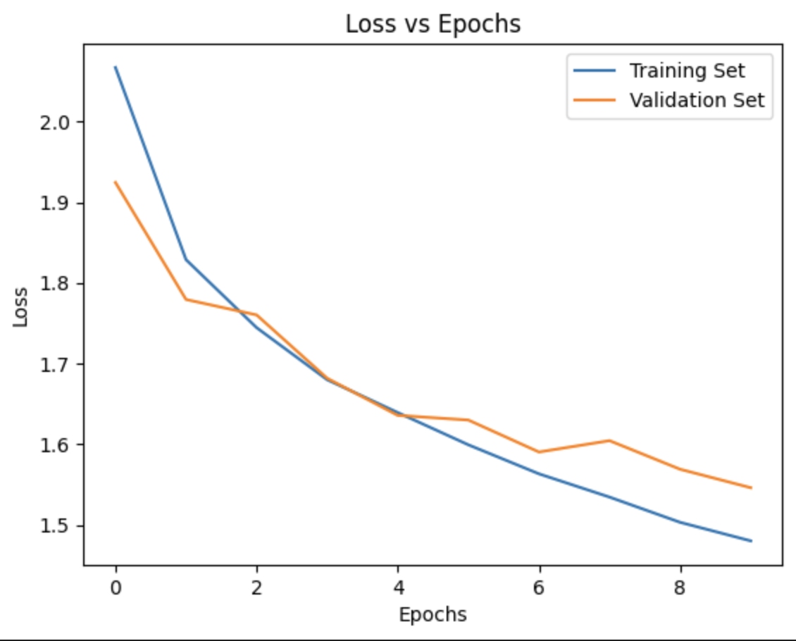
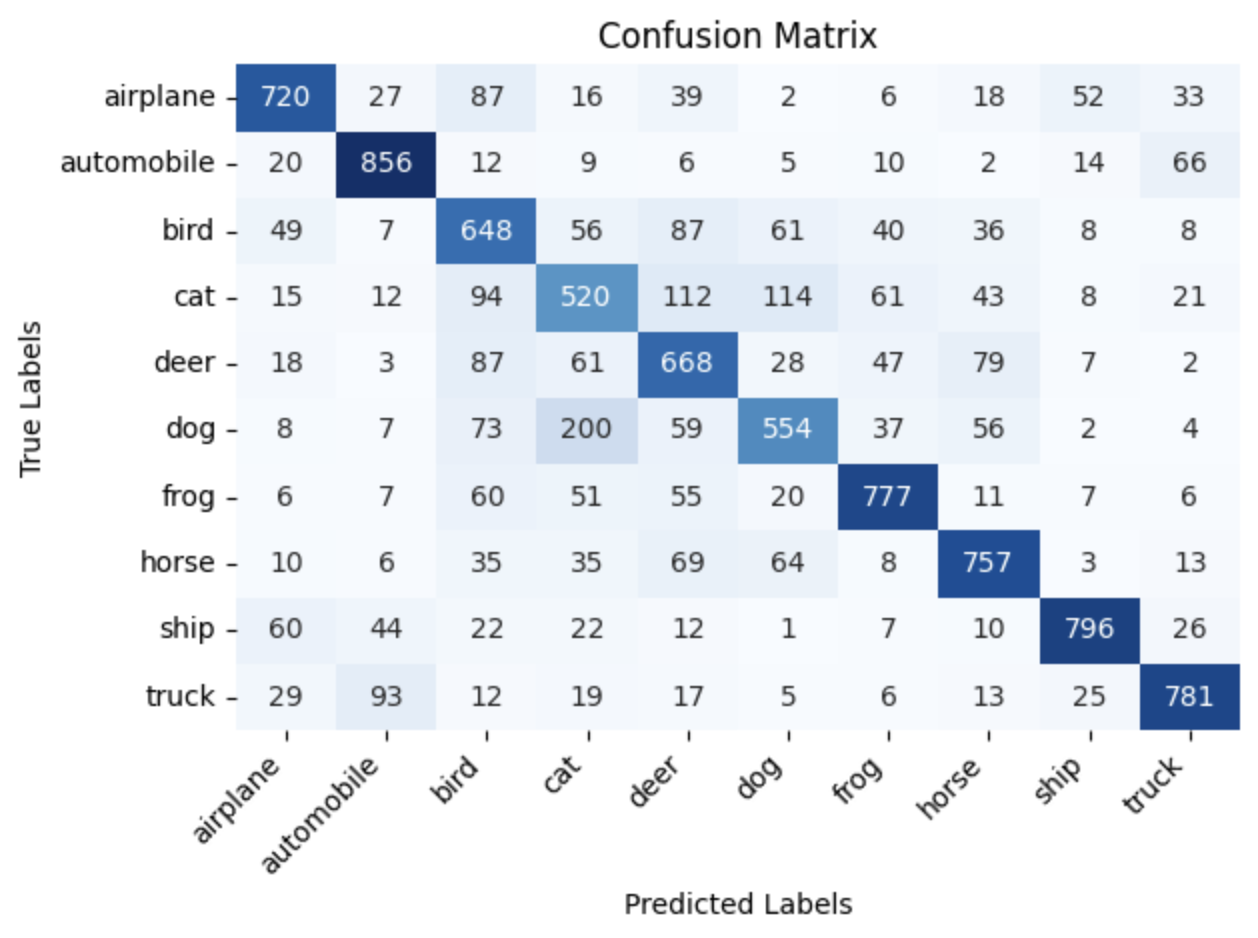
As expected, the performance of a simple deep NN for images is not really “state-of-the-art”, with a final accuracy of 46.8% on the training set and 44.7% on the validation set.

Judging from the confusion matrix, the largest mismatches occur between cats and frogs. There is also a significant confusion between cats and dogs, which is more understandable. However, some unpredictable mismatches appear between labels such as frogs and dogs, dogs and airplanes, and trucks and automobiles.

Other models, like CNNs, can capture the complexity of images in a much more effective manner.

Convolutional Neural Network

Now, let’s build a deep CNN to compare the performance of a more complex model. The feature extractor will consist of 3 convolutional layers, using max pooling to reduce the spatial dimensions of the features. The classifier, on the other hand, will contain 4 linear layers and use ReLU as the activation function.

class MyCNN(nn.Module):
  def __init__(self, in_ch, out_ch1, out_ch2, out_ch3, k_sz, nh1, nh2, nh3, no, stride):
    super().__init__()
    self.conv1 = nn.Conv2d(in_ch, out_ch1, k_sz, stride)
    self.conv2 = nn.Conv2d(out_ch1, out_ch2, k_sz, stride)
    self.conv3 = nn.Conv2d(out_ch2, out_ch3, k_sz, stride)
    self.linear1 = nn.Linear(out_ch3*2*2, nh1)
    self.linear2 = nn.Linear(nh1, nh2)
    self.linear3 = nn.Linear(nh2, nh3)
    self.linear4 = nn.Linear(nh3, no)

  def forward(self, x):
    x1 = F.max_pool2d(torch.relu(self.conv1(x)), 2)     # conv block 1
    x2 = F.max_pool2d(torch.relu(self.conv2(x1)), 2)    # conv block 2
    x3 = F.max_pool2d(torch.relu(self.conv3(x2)), 2)    # conv block 3
    x = x3.view(x3.size(0), -1)
    x = torch.relu(self.linear1(x))
    x = torch.relu(self.linear2(x))
    x = torch.relu(self.linear3(x))
    x = self.linear4(x)
    return x, x1, x2, x3

The training and validation losses evolved as such:

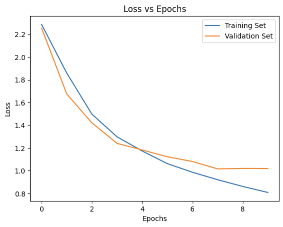
Already, we can observe that the CNN is performing significantly better, achieving 71.3% accuracy on the training set and 64.3% accuracy on the validation set, with no signs of overfitting.

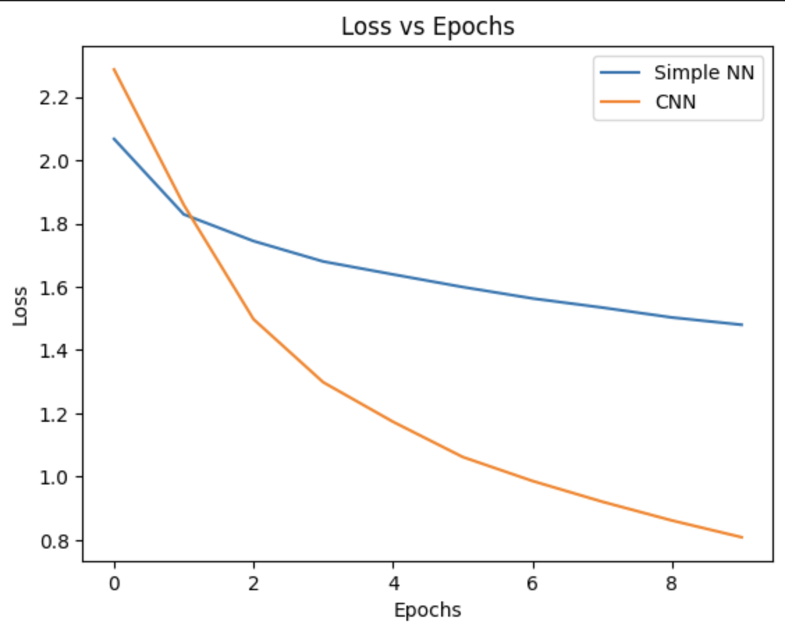
This graph compares the training loss of the simple NN and the CNN. It is clear that a more complex model like the CNN, which applies filters to the images, performs better, showing a steeper decrease in loss that becomes particularly noticeable around epoch 1.

More Epochs

So far, we’ve only trained for 10 epochs. What if we double that?

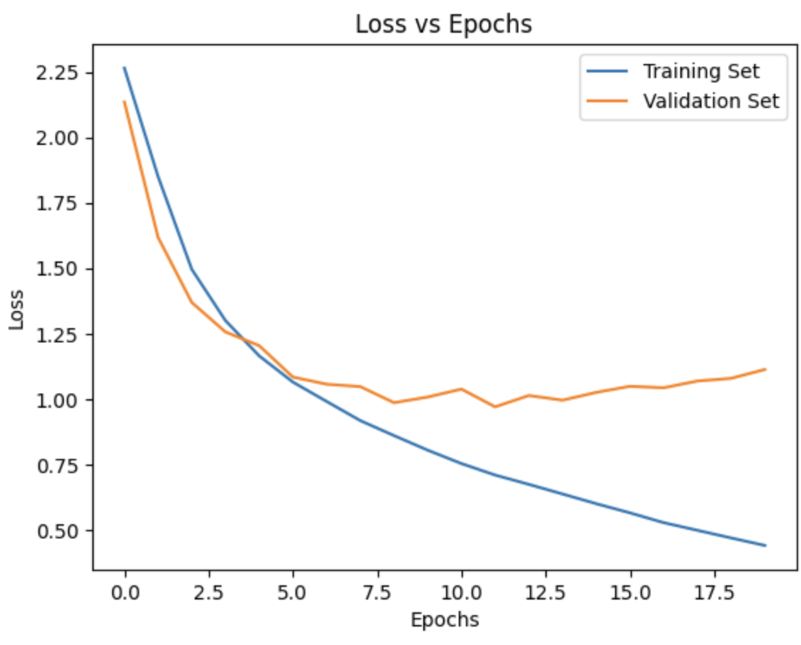
This graph provides a better understanding of how a model like this may overfit on the training set. Even though it performs well for the first 10 epochs, we can clearly see that around epoch 10, the gradient of the validation loss starts becoming positive, indicating the onset of overfitting.

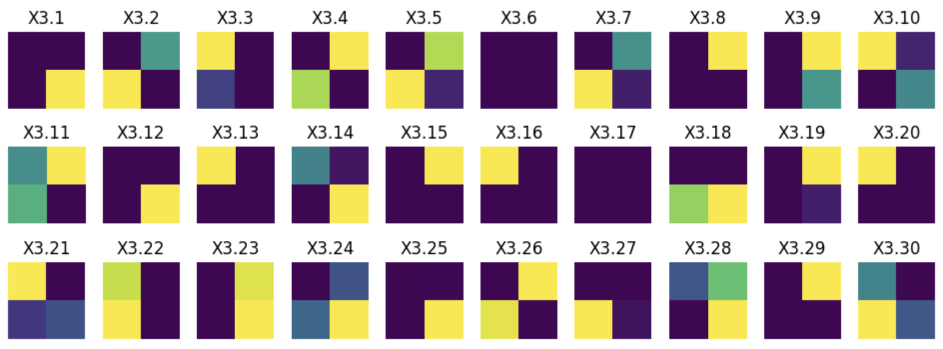
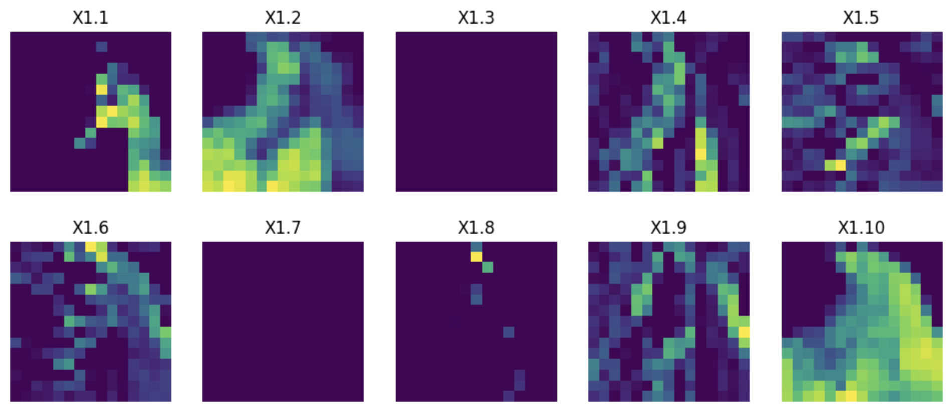
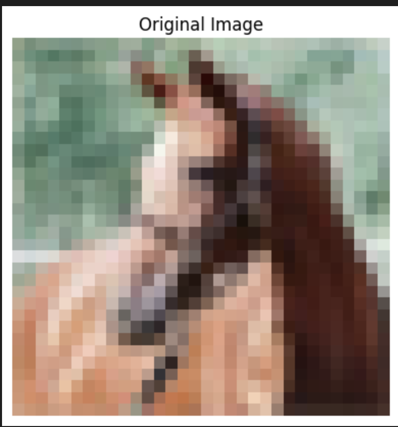
Bonus: These graphs show the intermediate features for the three convolutional layers. As observed, the first layers capture textures and edges, while deeper layers begin to identify more complex shapes (information dense receptive fields).

Data Augmentation

Data augmentation is a technique commonly used in machine learning to artificially expand a given dataset by applying various transformations to the existing data. It involves creating new training examples by making modifications to the original data, while preserving the label or class information.

The main goal of data augmentation is to increase the diversity and variability of the training data, which helps to improve the generalization and robustness of machine learning models. By exposing the model to a wider range of variations and patterns, it can learn more effectively and perform better on unseen or real-world data.

As we saw before, the model started overfitting when training for a higher number of epochs. Let’s apply some transformations to the data to check if we can solve this problem. These include random rotations, color jitters, and horizontal flips.

Note: We only apply the transformnations to the training set, as we want to leave the validation and testing sets as accurate to the actual images as possible.

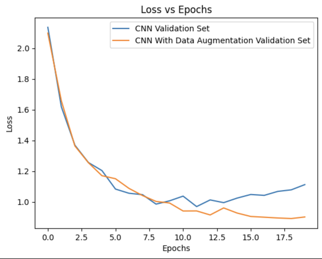
The validation loss is now performing better with data augmentation, achieving 69.7% accuracy and significantly mitigating the overfitting problem observed earlier.

Is this the best we can do? Certainly not. Pretrained models on much larger datasets can help address challenges like this, where smaller datasets do not provide enough information for the model to learn effectively.

Residual Network

Transfer learning means taking the relevant parts of a pre-trained machine learning model and applying it to a new but similar problem. Transfer learning brings a range of benefits to the development process of machine learning models. The main benefits of transfer learning include the saving of resources and improved efficiency when training new models. It can also help with training models when only unlabelled datasets are available, as the bulk of the model will be pre-trained.

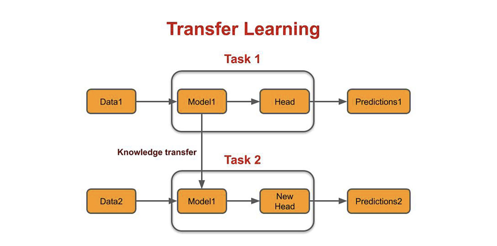
We will be using the ResNet-18 network pretrained on the ImageNet dataset. ImageNet contains millions of labeled images across a wide range of categories, including animals, objects, and scenes. The only fine-tuning performed here is on the final layer, as we need to adjust it to output predictions for the 10 labels in our dataset.

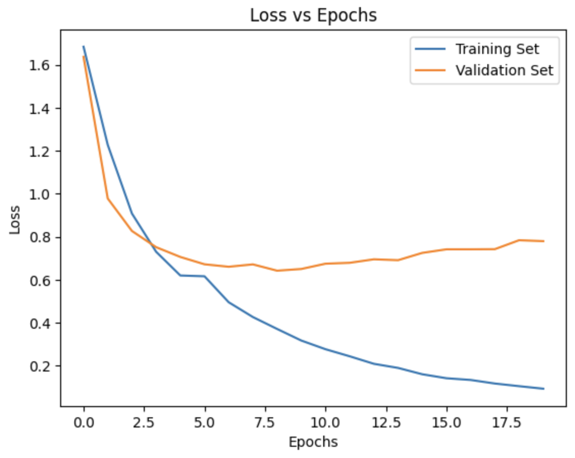
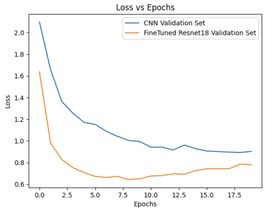
An increase in accuracy of around 10%! The starting loss is much smaller for the pretrained network for both the validation and training sets. Testing accuracy of 82.0%.

Now, the question arises once again: is this the best we can do? In many implementations, including the one in PyTorch, the default input size for the ResNet models is 224x224 pixels. But we are feeding it 32x32 images. Let’s fix this by resizing the images to 224x224.

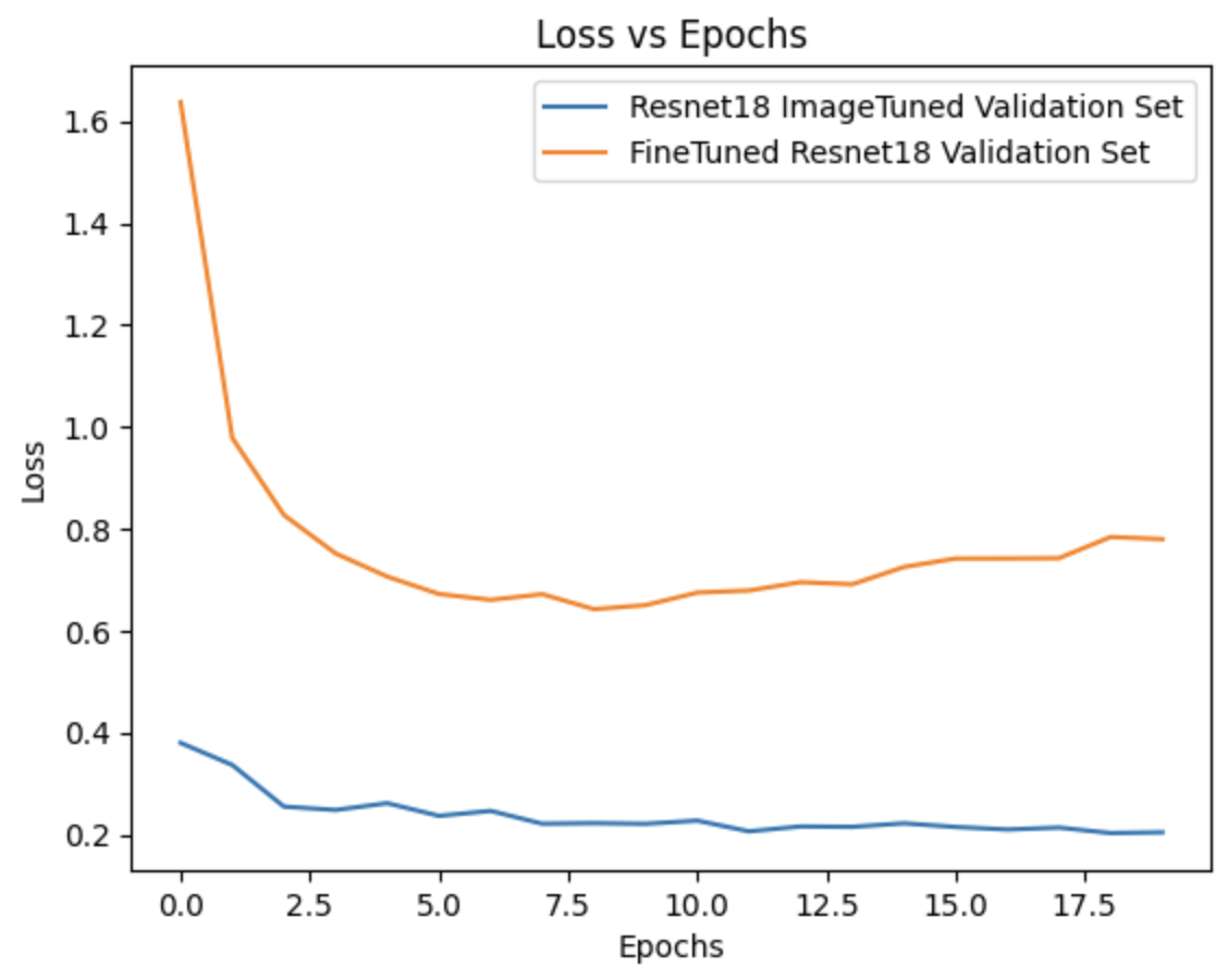
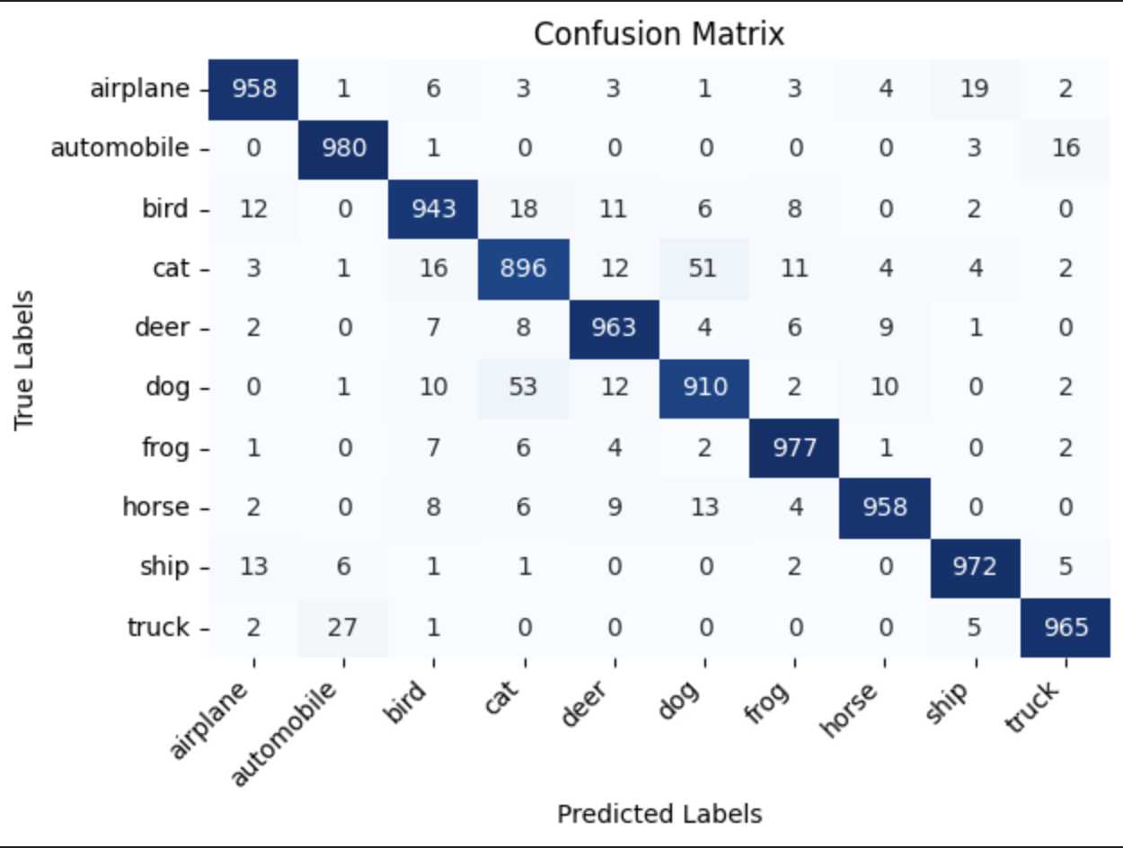
Now it’s clear that it wasn’t fair to feed the model differently sized images to the ones that were used to train it in the first place. Particularly, it is really impressive how low the loss starts for the validation set. Finally, we have a testing accuracy of 95%.